Running a plate based curvefit experiment

A guide to walk you from start to end. From importing the reader files to storing the curvefit results

Creating a plate from scratch

To create a new plate in a curve fit experiment, navigate to the “Plates” tab of an experiment that has the “curvefit” plugin and click the ”+” button in the toolbar.

Enter a name for the plate, its barcode, the type of plate and optionally a predefined plate layout, and click submit.

Notice: the barcode must be unique in the entire system, and you will encounter an error if the barcode is already in use.

Importing plate data

Plate data like counts, normalised values and concentrations can be imported into new or existing plates in an experiment from text files containing plate data arranged in the following format:

	01	02	03	04	05	…	XX
A	000	000	000	000	000	…	000
B	000	000	000	000	000	…	000
C	000	000	000	000	000	…	000
…	…	…	…	…	…	…	…
NN	000	000	000	000	000	…	000

To import plate data in the experiment, navigate to the “Plates” tab and click the “Import” button in the toolbar.

Drop or select the file you wish to import, and click “Next”.

You will be presented with the first bit of text in the file that the system has identified as a potential plate data. From there, you can choose to skip this bit of data, or add it to a new or existing plate in the experiment

If choosing to create a new plate, you will need to enter a name, a barcode and an optional plate layout.

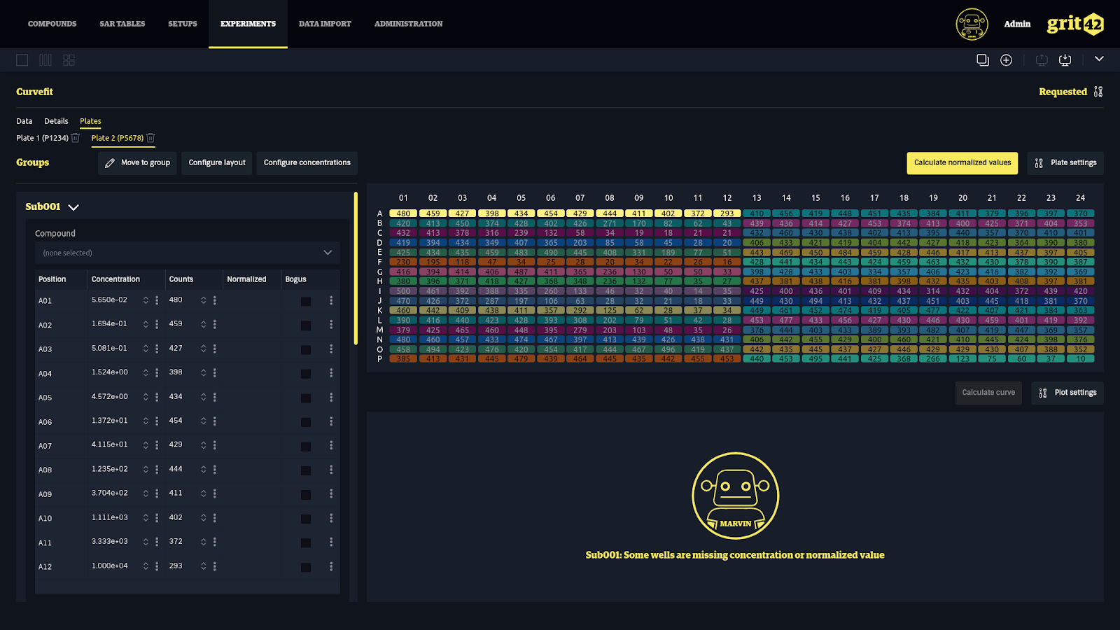
Configuring the plate layout

If no predefined plate layout matches, the plate layout can be configured in the experiment and saved for later. To configure the plate layout, simply select wells in the plate view and assign them a usage by clicking on the “Add to group” button if they have no usage yet, or “Move to group” otherwise.

Once the layout has been configured manually, it can be saved for future use by clicking the “Configure layout” button, then the “Save as new layout” button. 

Configure concentrations

Concentrations can be configured in bulk, for the whole plate or only selected wells by clicking the “Configure concentrations” button. The bulk configuration is based on the groups, and takes:

• a base concentration, which will be used for the first well in the group
• a dilution factor, which will be used to calculate subsequent concentration
• a dilution redundancy, which specifies the number of redundant concentrations (redundancy of 2 would mean there are 2 wells with the same concentration for each concentration in the group)
• a dilution direction, which will be used to identify the starting well for the process
  • Negative: start from the well closest to the bottom right of the plate
  • Positive: start from the well closest to the top left of the plate

Concentrations can also be configured for individual wells by selecting them in the plate view and editing the “concentration” field in the table to the left.

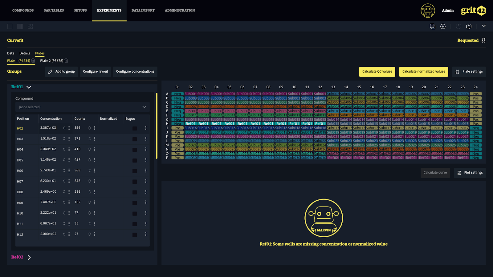
Plate quality control

When a plate has positive and negative control wells with counts defined, the system lets users calculate QC values (Z factor, window, positive and negative averages, standard deviations and relative standard deviations) by clicking the “Calculate QC values” button. Once these values are calculated, they can be controlled by clicking the “QC values” button, and may be recalculated from there.

 

If these values are off, users can select the wells that seem bogus and mark them as so in the table on the left. This will automatically refresh the QC values, as well as normalised values if possible. 

Normalisation

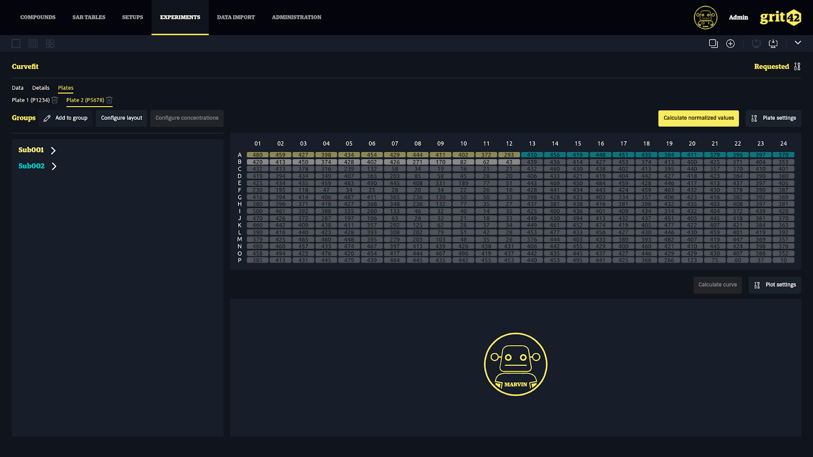
If there is a valid control source in the experiment (a plate with at least two negative and two positive non bogus controls with counts), users can calculate normalised values for the plate by clicking the “Calculate normalised values” button. If there are multiple valid control sources in the experiment, a list will appear and users can choose the control source to use for calculation.

If a control well is updated, normalised values will be automatically refreshed.

Linking subjects and compounds

To link compounds and subjects, select a subject in the list on the left and select a compound in the “Compound” dropdown above the table.

Once a compound has been selected, it will be linked in the results when the curves are calculated later.

Curve fitting

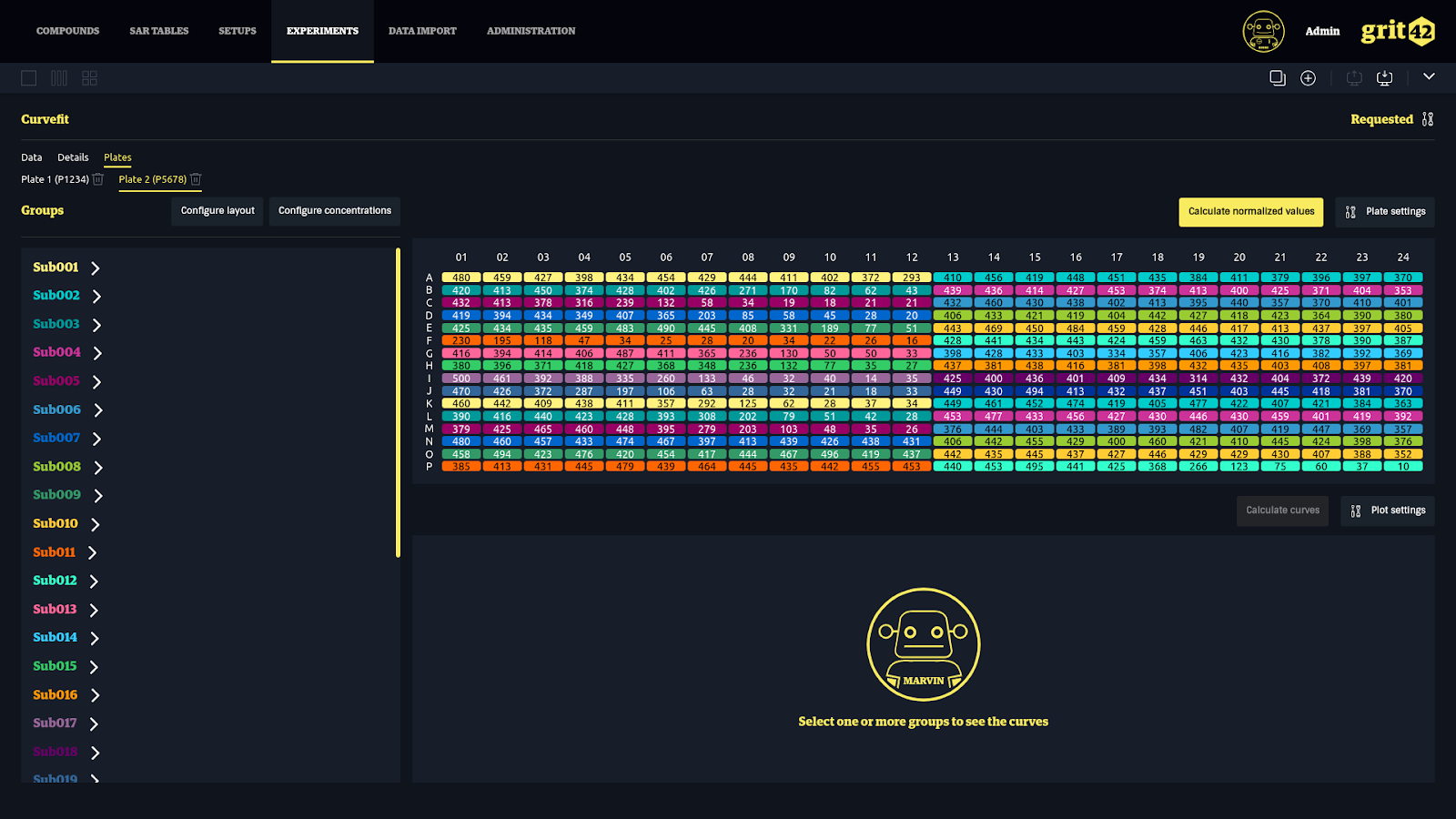
Calculating the curves

Once a plate has its layout and concentration defined, and normalised values defined or calculated, the curve values (min, max, v50 and slope) for each group can be calculated. To do so, click the “Calculate curves” button. 

Once the curves have been calculated, select a group in the list on the left to show its curve below the plate view.

Bogusing points

If a point is off, it can be marked as bogus by clicking it in the plot or its checkbox in the table to the left.

A bogus point will be shown in the plot with a cross instead of a dot.

Marking a point bogus will refresh the curve automatically. 

Fixing curve values

Min, max, v50 and slope can be overwritten. To do so, enter a new value in the appropriate field and the curve will refresh automatically.

To revert to the calculated value, edit the field again, leaving it blank.

Normalised-only mode

The curve fit plugin can be used in a “normalised values only” mode, when the counts are not available. The switch to this mode is automatic when wells have normalised values without counts.

In normalised-only mode, users can still bogus points and calculate curve values, but won’t be able to see QC values. Bogusing controls will have no effect, as the system is not able to calculate normalised values.

Experiment results

Calculated curve values are saved as results for the experiment and can be found under the “Data” tab of the experiment. 

Curve fit experiment results include: 

• The subject name
• The linked compound, if any
• The calculated min, max, v50 and slope values
• The fixed min, max, v50 and slope values